1D Distributions

The datasets that can be plotted are given in Datasets.

Commandline

1D distributions can be plotted using plot_1d_dist. This can be run from the command line with:

python plot_1d_dist.py

Options can be determined by appending --help to the call.

Example commandline calls are given below with the code examples.

Code

A plot of the 1D distribution for a single parameter for single dataset can be done using the code below.

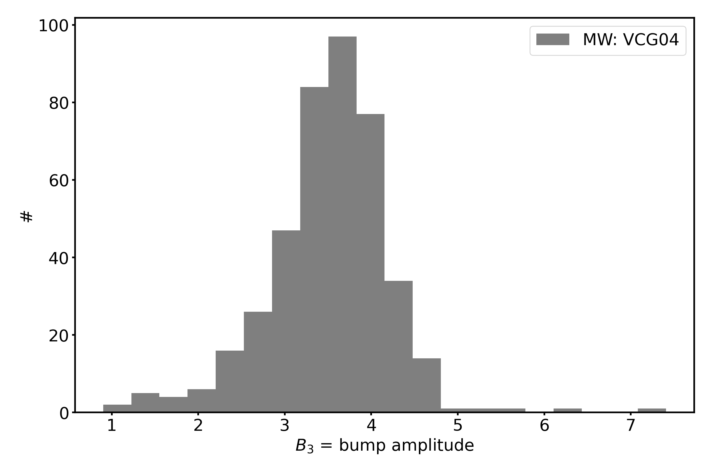
Example 1

This shows an example for the VCG04 sample of Milky Way sightlines for the FM90 parameter B3.

import matplotlib.pyplot as plt
from extinction_ensemble_props.plot_1d_distributions import plot_1d_dist

fontsize = 20
font = {"size": fontsize}
plt.rc("font", **font)
plt.rc("lines", linewidth=2)
plt.rc("axes", linewidth=2)
plt.rc("xtick.major", width=2)
plt.rc("ytick.major", width=2)

fsize = (12, 8)
fig, ax = plt.subplots(figsize=fsize)

plot_1d_dist(ax, ["VCG04"], "B3")

fig.tight_layout()
plt.show()

(Source code, png, hires.png, pdf)

The equivalent commandline call is:

python extinction_ensemble_props/plot_1d_distributions.py --param B3 --datasets VCG04

Example 2

This shows an example for the VCG04, FM07, and GCC09 samples of Milky Way sightlines for the FM90 parameter C2 now including Gaussian fits to each sample.

import matplotlib.pyplot as plt
from extinction_ensemble_props.plot_1d_distributions import plot_1d_dist

fontsize = 20
font = {"size": fontsize}
plt.rc("font", **font)
plt.rc("lines", linewidth=2)
plt.rc("axes", linewidth=2)
plt.rc("xtick.major", width=2)
plt.rc("ytick.major", width=2)

fsize = (12, 8)
fig, ax = plt.subplots(figsize=fsize)

plot_1d_dist(ax, ["VCG04", "FM07", "GCC09"], "B3", fit=True)

fig.tight_layout()
plt.show()

(Source code, png, hires.png, pdf)

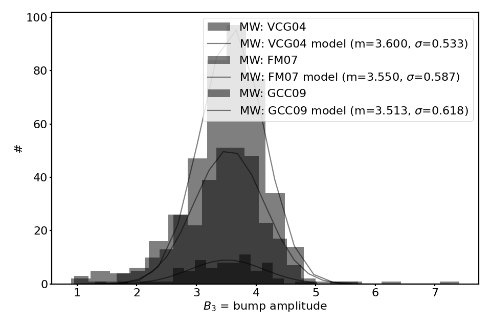
The equivalent commandline call is:

python extinction_ensemble_props/plot_1d_distributions.py --param C2 --datasets VCG04 FM07 GCC09 --fit

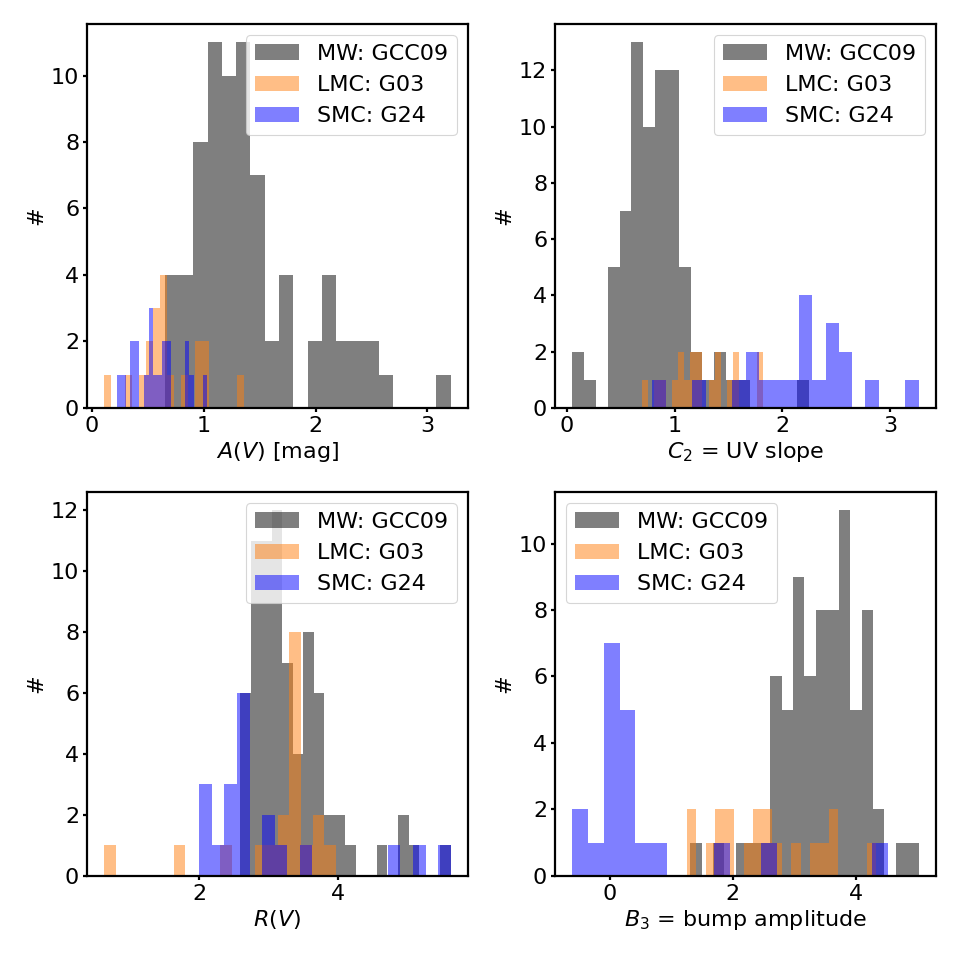
Example 3

This shows how to make a set of plots showing different 1D distributions for multiple datasets. One dataset from the Milky Way (GCC09), LMC (G03_lmc), and SMC (G24_smc) are used.

import matplotlib.pyplot as plt
from extinction_ensemble_props.plot_1d_distributions import plot_1d_dist

fontsize = 20
font = {"size": fontsize}
plt.rc("font", **font)
plt.rc("lines", linewidth=2)
plt.rc("axes", linewidth=2)
plt.rc("xtick.major", width=2)
plt.rc("ytick.major", width=2)

fsize = (12, 12)
fig, ax = plt.subplots(nrows=2, ncols=2, figsize=fsize)

datasets = ["GCC09", "G03_lmc", "G24_smc"]
plot_1d_dist(ax[0, 0], datasets, "AV")
plot_1d_dist(ax[1, 0], datasets, "RV")
plot_1d_dist(ax[0, 1], datasets, "C2")
plot_1d_dist(ax[1, 1], datasets, "B3")

fig.tight_layout()
plt.show()

(Source code, png, hires.png, pdf)

There is no commandline equivalent.